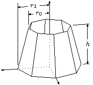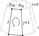

Let's look at a drawing that represents the kind of problem
sketch was meant to solve—a pair of textbook figures
regarding a polygonal approximation of a truncated cone. Here are the
pictures we will produce.


The cone shape is just a swept line with no closure tag and culling turned off. Begin by setting up some useful constants.
  def O (0,0,0) def I [1,0,0] def J [0,1,0] def K [0,0,1]
  def p0 (1,2) def p1 (1.5,0) def N 8
  def seg_rot rotate(360 / N, [J])
The points
p0 and p1 are the end points of the line to
be swept. The definition seg_rot is the sweep transformation.
With these, the cone itself is simple.
sweep[cull=false] { N, [[seg_rot]] } line(p0)(p1)
The axes are next and include an interesing trick that shows the
hidden parts as dotted lines. The secret is draw the axes
twice—solid lines with the normal
hidden surface algorithm in effect, and then dotted with the
option
lay=over so that no polygons can hide them.
  def ax (dx,0,0) % tips of the axes
  def ay (0,dy,0)
  def az (0,0,dz)
  line[arrows=<->,linewidth=.4pt](ax)(O)(ay)
  line[arrows=->,linewidth=.4pt](O)(az)
  % repeat dotted as an overlay to hint at the hidden lines
  line[lay=over,linestyle=dotted,linewidth=.4pt](ax)(O)(ay)
  line[lay=over,linestyle=dotted,linewidth=.4pt](O)(az)
  special|\footnotesize
          \uput[d]#1{$x$}\uput[u]#2{$y$}\uput[l]#3{$z$}|
    (ax)(ay)(az)
The labels are applied with PSTricks special objects
as usual.
For the height dimension mark, the power of affine arithetic is very helpful.
  def hdim_ref unit((p1) - (O)) then [[seg_rot]]^2
  def c0 (p0) then scale([J])
  def h00 (c0) + 1.1 * [hdim_ref]
  def h01 (c0) + 1.9 * [hdim_ref]
  def h02 (c0) + 1.8 * [hdim_ref]
  line(h00)(h01)
  def h10 (O) + 1.6 * [hdim_ref]
  def h11 (O) + 1.9 * [hdim_ref]
  def h12 (O) + 1.8 * [hdim_ref]
  line(h10)(h11)
  line[arrows=<->](h02)(h12)
  def hm2 ((h02) - (O) + (h12) - (O)) / 2 + (O)
  special|\footnotesize\rput*#1{$h$}|(hm2)
The general idea employed here is to compute a unit “reference
vector” parallel to the xz-plane in the desired direction of
the dimension from the origin. The transformation
[[seg_rot]]^2 rotates two segments about the y-axis.
When applied to (p1) - (O), the resulting vector points to the
right as shown. In this manner, we can pick any vertex as the
location of the height dimension lines by varying the exponent of
[[seg_rot]]. This is only one of many possible strategies.
The computation of hm2 is a useful idiom for finding the
centroid of a set of points.
The two radius marks are done similarly, so we present the code without comment.
  % radius measurement marks
  def gap [0,.2,0]  % used to create small vertical gaps

  % first r1
  def up1 [0,3.1,0] % tick rises above dimension a little
  def r1 ((p1) then [[seg_rot]]^-2) + [up1]
  def r1c (r1) then scale([J])
  def r1t (r1) + [gap]
  def r1b ((r1t) then scale([1,0,1])) + [gap]
  line[arrows=<->](r1c)(r1)  % dimension line
  line(r1b)(r1t)             % tick
  def r1m ((r1) - (O) + (r1c) - (O)) / 2 + (O) % label position
  special |\footnotesize\rput*#1{$r_1$}|(r1m)  % label

  % same drill for r0, but must project down first
  def up0 [0,2.7,0]
  def r0 ((p0) then scale([1,0,1]) then [[seg_rot]]^-2) + [up0]
  def r0c (r0) then scale([J])
  def r0t (r0) + [gap]
  def r0b ((p0) then [[seg_rot]]^-2) + [gap]
  line[arrows=<->](r0c)(r0)
  line(r0b)(r0t)
  def r0m ((r0) - (O) + (r0c) - (O)) / 2 + (O)
  special |\footnotesize\rput*#1{$r_0$}|(r0m)
The second drawing uses the same techniques. Only the method for drawing the elliptical arc is new. Here is the code.
  def mid ((p00)-(O)+(p10)-(O)+(p11)-(O)+(p01)-(O))/4+(O)
  special|\rput#1{\pscustom{
    \scale{1 1.3}
    \psarc[arrowlength=.5]{->}{.25}{-60}{240}}}|
    [lay=over](mid)
We could have swept a point to make the arc with sketch, but
using a PSTricks custom graphic was simpler. Again we computed
the
centroid of the quadrilateral by averaging points. Note that scaling
in Postscript distorts the arrowhead, but in this case the distortion
actually looks better in the projection of the slanted face. A
sketch arrowhead would not have been distorted.
The complete code for this example, which draws either figure
depending on the definition of the tag <labeled>, is included
in the sketch distribution in the file truncatedcone.sk.